Research - (2020) Volume 9, Issue 6
A modern approach in the area of nanotechnology for collection of information and solving physical problems is the utilization of nanoparticles. The area of solar power generation and heat exchanger in industrial zone have been redeveloped and modernized due to the utilization of nanotechnology. By utilizing nanotechnology, the area of pharmaceutical Science has been re-developed and modernized. The use of nanotechnology in medicine as well as pharmaceutical industries has attracted scientists to develop more modern and economical applications. Remembering these brightful applications, a numerical simulation for Arrhenius activation energy and binary chemical aspects in Cross nano fluid past a cylinder has been presented here. A recently proposed nano fluid model (Buongiorno’s model) is utilized to account Brownian diffusion and thermophoresis. Additionally, velocity slip condition is implemented. Furthermore, time dependent magnetic effects are taken into account. Salient influences of binary chemical aspects and activation energy are also considered in concentration equation. We achieved highly nonlinear differential system. The numerical simulation of such highly nonlinear system is not an easy task. We utilized Shooting Runge-Kutta Fehlberg (RK45) approach to tackle this highly nonlinear problem. The escalating values of chemical reaction rate parameter and temperature difference parameter decline the concentration of nanoparticles. Reduction in rate of mass transfer is revealed against activation energy parameter. Accelerating behavior is observed in Nusselt number for larger estimation of unsteadiness parameter and velocity slip parameter. Fluid temperature is accelerated against thermophoresis parameter. Surface drag force grows for larger Wiesenberger number
Arrhenius activation energy, Binary chemical reactions, Cross nano fluid, MHD.
Mechanism of flow in the regions of high and low shear rates as well as power law region has a great impact on practical applications in industrial and engineering fields. Investigators and scientists are interested to adopt such a model which has the characteristics to depict the flow in these regions. Cross viscosity model is an important class of (GNF) generalized Newtonian fluid that has a quality to depict the flow in low shear rate region, power law region and high shear rate region [1]. This model demonstrates stress characteristics. Due to the involvement of time constant in the Cross rheological model, the importance of this model has enhanced for industrial and engineering computations. This model has many applications such as 0:4% aqueous solution for polyacrylamide, aqueous solution for polymeric latex sphere, synthesis for polymeric solutions, blood and 0:35% aqueous solution for Xanthan gum [2]. The experimental investigation of Cross rheological model was initiated by Escudier et al. [3]. They expressed the storage and loss moduli as well as viscometric viscosity. Xie and Jin studied Cross rheological model and they utilized WC-MPS method to depict four parameters of Cross rheological model [4]. Recently, Azam, et al. conducted a numerical simulation of Cross nano fluid with nonlinear radiation for the case of a sheet [5]. Their numerical analysis reveals that nanoparticles concentration field was depressed for higher values of Brownian motion parameter. The flow analysis past a moving cylinder has been a subject of demanding research from the last decade. The formulation of cylinder-like structures during blunt-body flows and the related heat transfer mechanism has concrete applications in several engineering and industrial relevance such as formation of heat exchanger tube, cooling towers, chimney stacks and offshore structure. Understanding of heat transfer mechanism plays a key role in formation of instruments utilizing wires and hot wire anemometers. Investigations depict that the wake structure unsettled and hydrodynamic instabilities enhance when the wake is affected by solutal or thermal buoyancy. Uchida and Aoki initiated the work of unsteady flows in a pipe with contracting or expanding walls [6]. They achieved single 4th order differential equation from the flow equation. Steady flow of viscous liquid on outside contracting or expanding cylinder was firstly proposed by Wang [7]. Transient flow of viscous fluid outside the expanding/contracting cylinder was studied by Fang et al. [8]. They noted that there is no axial flow for trivial solution. A numerical study for Carreau nano fluid flow over a cylinder was presented by Azam et al. [9]. They depicted that momentum layer thickness diminished for enhancing Wiesenberger number. Jourabian et al. discussed melting process in porous cylinders [10]. They utilized Lattice Boltzmann approach to execute numerical analysis. Sheikholeslami presented a novel computational approach to analyzed entropy in nano fluid [11]. He also used the effects of energy in this study.
Svante Arrhenius proposed the concept of activation energy in 1889. He aimed to achieve energy from chemical reactions known as activation. The minimum energy that is required to initiate any chemical reaction process is called activation energy. It is generally used in medicines, oil, water and oil emulsions. Bestman was the best who introduce chemical process in boundary layer [12]. He discussed activation energy impact in convective flow and solved the work via perturbation technique. Makinde et al. studied chemically reacting flow over a porous surface [13]. They also considered the impact of thermal radiation in this investigation. Abbas et al. investigated binary chemical process in radiative flow of Casson fluid [14]. They noted that solute boundary layer depreciated for growing values of chemical reaction rate parameter. Sandeep studied magnetic nano fluid with graphines nanoparticles [15]. For numerical solutions, he used Runge-Kutta Method. Hsiao presented activation energy aspects in Carreau nano fluid. He used parameters control approach to find solution of considered study [16]. Ijaz and Nadeem presented an article to examine blood related nanoparticles transportation across atherosclerotic artery [17]. In their investigation, hemodynamics of atherosclerotic artery uplifted. Recently, Azam et al. worked on activation energy in Cross nano fluid with binary chemical reactions [18]. They noted that augmentation in activation energy parameter resulted in larger nanoparticles concentration.
Existing study pointed out that numerical simulation for arrhenius activation energy and binary chemical aspects in transient slip flow of magneto-Cross nano fluid over a moving cylinder is not investigated yet. The main focus of this attempt is to examine the impact of activation energy on transient slip flow of Cross nano fluid with binary chemical reaction. The fluid is assumed to be flowing outside the cylinder. Buongiorno’s nano fluid model is utilized for the suspension of nanoparticles. Time magnetic field is also contributed. The partial differential system is altered into ordinary differential system by utilizing boundary layer approximation and suitable transformations. Shooting RK45 numerical technique is utilized to solve this highly nonlinear differential system. Numerical computations for mass transfer rate, Nusselt number and drag surface force are also executed in tables. Additionally, impact of pertinent variable on nanoparticles concentration, temperature and velocity fields are demonstrated graphically. A comparative analysis with existing research is conducted and achieved in excellent agreement.
A mathematical modeling for unsteady incompressible two dimensional chemically reacting flow of Cross nano fluid over a shrinking cylinder subject to arrhenius activation energy is conducted. The unsteady radius of cylinder is modeled as

Where a0 is positive constant possessing dimension length, the constant of contraction/expansion strength and t the time. The unsteady radius of cylinder decreases with time for β>0 and while it enhances for β<0. The x- and r- axes are directed along axial and radial ways respectively. A non-uniformly transverse magnetic Field applied to radial direction is expressed as

Where B0 is intensity of magnetic field. The induced magnetic field is neglected due to assuming small enough Reynolds number. The cylinder surface is at constant temperatureTw and constant nanoparticle concentration Cw. Also we assumed that T∞ and C∞ are ambient fluid temperature and concentration respectively such that Tw>T∞ and Cw>C∞. Additionally, velocity slip condition is applied at surface of cylinder. The mathematical expression for velocity partial slip condition in Cross fluid is modeled as

Where l is slip length possessing dimension of length and Γ is time constant.
For the contribution of thermophoresis and Brownian motion, Buongiorno’s nano fluid model is adopted. The cylinder can stretch or shrink with time dependent velocity which is linear proportional to axial distance from origin. This time dependent velocity is expressed in such a way

Where v is momentum diffusivity.
The stress tensor for four parameter fluid can be stated as

Where I is identity tensor, p the pressure, A1 the first Rivlin Ericksen tensor which is written as

in which ▽V is velocity gradient. μ is apparent viscosity.
The rheology equation for Cross fluid (1) (sub class of generalized Newtonian fluid) can be demonstrated as

Where μ0 and μ∞ are infinity shear rate and zero shear rate viscosities respectively, n the power law index and γ is shear rate that can be expressed as

In present study, we take μ∞ = 0 then stress tensor modified to

Note that Cross fluid can be recover to Newtonian model when Γ = 0.
In cylindrical coordinates the velocity, temperature as well as nanoparticles concentration field are stated as

With the application of boundary layer dynamism and assumptions, the equations of continuity, momentum, and energy and nanoparticles concentration are listed below

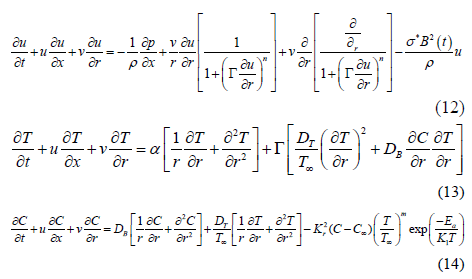
Boundary conditions

where is α thermal diffusivity, DT thermophoresis diffusion
coefficient,  ratio of heat capacity of
nanoparticles to heat capacity of base fluid, DB Brownian
diffusion coefficient, ρ fluid density, Kr chemical reaction rate
constant, Ea activation energy,
 modified
arrhenius function, K1 Boltzmann constant and m exponent
fitted rate constant.
We consider non-dimensional suitable transforming variables listed below

On putting Equation (17) into Equations (11)-(16), the equation of continuity is automatically satisfied and rest of highly nonlinear PDEs are reduced to the following ordinary differential system that is also highly nonlinear as given below.
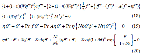
Non-dimensional boundary conditions

The mathematical expressions for non-dimensional parameters involved in above equations are listed below
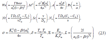
The above parameters are respectively named as Weissenberg number We, magnetic parameter M. unsteadiness parameter A, Prantdl number Pr, thermophoresis parameter Nt, Schmidt number Sc, Brownian motion parameter Nb, chemical reaction rate parameter σ, temperature difference parameter δ, activation energy parameter E and velocity slip parameter L.
Surface drag force
Mathematically, surface drag force (skin friction coefficient) is stated as

Where Trx indicates wall shear stress which is defined as

Putting Equation (25) in Equation (24) we get the resulting equation in the form

Heat transfer rate

Where qw represents wall heat flux which is defined as

Invoking Equation (28) in Equation (27) we get the reduced equation

Mass transfer rate
Mathematically, mass transfer rate (Sherwood number) is demonstrated as

where qm deals the wall mass flux which is defined as

Indorsing Equation (31) in Equation (30) we get the following expression

Current section is constructed to demonstrate the characteristics of comparative analysis, fluid velocity, Nusselt number, temperature field, Sherwood number, streamlines, nanoparticles concentration field, isotherms and skin friction coefficients through tables and graphs (Tables 1-4) and (Figures 1-11).
| L | Wang and Ng [19] | Abbas et al. [20] | Khan et al. [21] | Current study |
|---|---|---|---|---|
| 0 | -1.1778 | -1.7860 | -1.17884 | -1.17999 |
| 0.1 | -1.0116 | -1.068 | -1.01365 | |
| 0.5 | -0.6638 | -0.664 | -0.66542 | |
| 1 | -0.4739 | -0.4743 | -0.47502 | |
| 2 | -0.3070 | -0.3073 | -0.30743 | |
| 5 | -0.1532 | -0.1534 | -0.15345 | |
| 10 | -0.0848 | -0.085 | -0.08502 | |
| 20 | -0.4536 | -0.04536 | ||
| 30 | -0.031 | -0.03116 | ||
| 50 | -0.021 | -0.01921 | ||
| 70 | -0.01382 | |||
| 100 | -0.00976 |
Table 1: A comparison analysis of f″(1) for some values of L in case of stretching cylinder (f′(1)=1) when We=M=A=0.0 and n=1.0.
| Parameters | Skin friction coefficient | |||
|---|---|---|---|---|
| A | L | We | M |  |
| 1 | 0.5 | 0.2 | 0.5 | 0.24578 |
| 1.3 | 0.31875 | |||
| 1.6 | 0.35916 | |||
| 1 | 1 | 0.26451 | ||
| 1.4 | 0.26229 | |||
| 1.8 | 0.25142 | |||
| 0.8 | 0.1 | 0.27588 | ||
| 0.3 | 0.24888 | |||
| 0.5 | 0.23166 | |||
| 0.2 | 1 | 0.45285 | ||
| 1.5 | 0.58694 | |||
| 2 | 0.68388 | |||
Table 2: Numerical variation of  for some values of A,
L, We, M when n=0.6.
| Parameters | Nusselt number | ||||
|---|---|---|---|---|---|
| A | L | M | Nb | Nt | -θ′(1) |
| 1 | 0.00519 | ||||
| 1.3 | 0.00532 | ||||
| 1.6 | 0.00668 | ||||
| 1 | 1 | 0.00775 | |||
| 1.5 | 0.01039 | ||||
| 2 | 0.01271 | ||||
| 0.5 | 1 | 0.01105 | |||
| 1.4 | 0.01517 | ||||
| 1.8 | 0.01824 | ||||
| 1 | 0.2 | 0.01053 | |||
| 0.3 | 0.01003 | ||||
| 0.4 | 0.00956 | ||||
| 0.1 | 0.2 | 0.0025 | |||
| 0.3 | 0.00238 | ||||
| 0.4 | 0.00226 |
Table 3: Numerical variation of -θ′(1) for some values of A, L, M, Nb, Nt and n when Pr=0.71;,m=Sc=1.0, We=0.2 and n=0.6.
| Parameters | Sherwood number | ||||||||
|---|---|---|---|---|---|---|---|---|---|
| A | L | M | Nb | Nt | Sc | δ | E | σ | -θ′(1) |
| 1 | 0.8 | 0.8 | 0.1 | 0.1 | 1 | 0.5 | 0.5 | 0.5 | 0.392385 |
| 1.3 | 0.324801 | ||||||||
| 1.6 | 0.27772 | ||||||||
| 1 | 1 | 0.39771 | |||||||
| 1.5 | 0.40854 | ||||||||
| 2 | 0.41646 | ||||||||
| 1 | 1 | 0.40622 | |||||||
| 1.5 | 0.42198 | ||||||||
| 1.8 | 0.42846 | ||||||||
| 1 | 0.2 | 0.38764 | |||||||
| 0.3 | 0.38664 | ||||||||
| 0.4 | 0.38615 | ||||||||
| 0.1 | 0.2 | 0.39609 | |||||||
| 0.3 | 0.40106 | ||||||||
| 0.4 | 0.40559 | ||||||||
| 0.1 | 0.5 | 0.38828 | |||||||
| 1.3 | 0.40306 | ||||||||
| 2 | 0.42534 | ||||||||
| 0.9 | 0.2 | 0.30089 | |||||||
| 1 | 0.51777 | ||||||||
| 1.5 | 0.63672 | ||||||||
| 1 | 1 | 0.42547 | |||||||
| 1.5 | 0.34764 | ||||||||
| 2 | 0.28268 | ||||||||
| 0.3 | 0.3 | 0.37408 | |||||||
| 0.7 | 0.71805 | ||||||||
| 1 | 0.92387 | ||||||||
Table 4: Numerical variation of -θ′(1) for some values of A, L, M, Nb, Nt, Sc, δ, E and σ with Pr=0.71, m=1.0, We=0.2 and n=0.6.
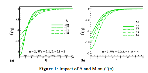
Figure 1: Impact of A and M on f ’(η).
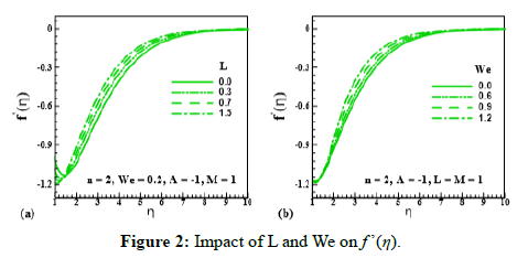
Figure 2: Impact of L and We on f ’(η).
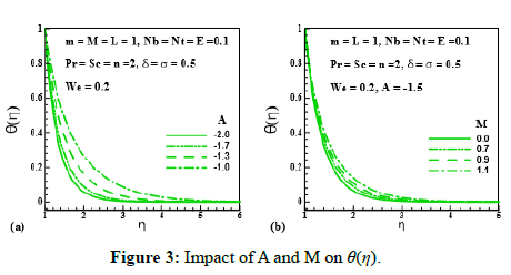
Figure 3: Impact of A and M on θ(η).
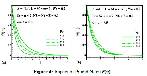
Figure 4: Impact of Pr and Nt on θ(η).
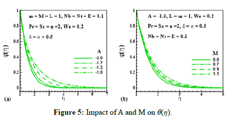
Figure 5: Impact of A and M on θ(η).
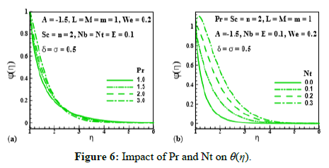
Figure 6: Impact of Pr and Nt on θ(η).
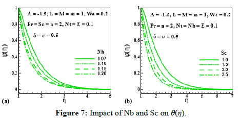
Figure 7: Impact of Nb and Sc on θ(η).
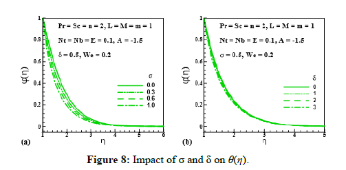
Figure 8: Impact of σ and δ on θ(η).
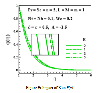
Figure 9: Impact of E on θ(η).
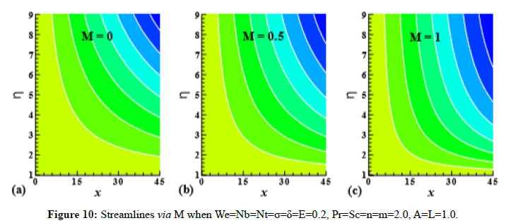
Figure 10: Streamlines via M when We=Nb=Nt=σ=δ=E=0.2, Pr=Sc=n=m=2.0, A=L=1.0.
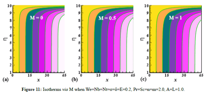
Figure 11: Isotherms via M when We=Nb=Nt=σ=δ=E=0.2, Pr=Sc=n=m=2.0, A=L=1.0.
Declaration of curiosity
Table 1 is formulated to ensure the guarantee of present
investigation with the comparative analysis of existing
work. From this table, it can be decided that our results are
in excellent agreement with the existing work. Table 2 is
constructed to depict the characteristics of (A), (L), (We) and
(M) on  when n=0.6 is fixed. Through this table, it can be clearly concluded that skin friction elevated for higher
values of (A) and (M). Additionally, surface drag force is
reduced for larger values of (L) and (We). Table 3 represents
the variation of –ϕ’(1) for different values of (A), (L), (M),
(Nb) and (Nt) when Pr=0:71, m=Sc=1:0, We=0.2 and n=0.6 are
fixed. On behalf of this table, it is easy to say that –ϕ’(1) is an
enhancing function of (A), (L) and (M). It is also predicted that –ϕ’(1) depreciates for growing values of (Nb) and (Nt). Table
4 demonstrates the effects of (A), (L), (M), (Nb), (Nt), (Sc),
(δ), (E) and (σ) on –ϕ’(1) when Pr=0.71, m=1.0, We=0.2 and
n=0.6 are fixed. Through this table, it is confirmed that –ϕ’(1) is
an uplifting function of (Nt), (M), (L), (Sc), (δ) and (σ). It is also
elucidated that –ϕ’(1) is diminished for higher estimation of (A),
(Nb) and (E).
Velocity distribution
Influence of unsteadiness parameter (A), magnetic parameter (M); velocity slip parameter (L) and Wiesenberger number (We) unsteadiness parameter (A), magnetic parameter (M), velocity slip parameter (L) and Wiesenberger number (We) on the velocity field is shown in Figure 1 and Figure 2 respectively. For higher estimation of (A= -2.0,1.7,1.3,1.0), velocity distribution (f’ (η)). reduces. It means, unsteadiness possesses a tendency to reduce fluid velocity. It is also examined that velocity distribution (f’ (η)). depreciates for higher estimation of (M=0.0,0.5,0.7,1.0): As (M) is directly proportional to resistive force (Lorentz force) which enhances the resistance inside fluid particles. As a result, (f’ (η)). decreases. Figure 2 elucidates the salient characteristics of (L) and (We) on the motion of fluid particles. It is observed that fluid velocity and its related layer thickness uplifts for upgrading estimation of (L=0.0,0.3,0.7,1.5). It is also indicated that velocity grows for larger estimation of (We=0.0,0.6,0.9,1.2). Physically, improvement in relaxation time causes in enhancement of (f’ (η)).
Temperature distribution
Figure 3 and Figure 4 reveal the behavior of unsteadiness parameter (A), magnetic parameter (M), Prantdl number (Pr) and thermophoresis parameter (Nt) on temperature distribution(θ (η)). Figure 3a indicates the enhancing behavior of temperature field (θ (η)) via unsteadiness parameter (A=2.0,1.7,1.3,1.0). This means unsteadiness tends to enhance temperature distribution (θ (η)). From Figure 3b temperature distribution (θ (η)) and its related layer thickness represent the improving behavior through magnetic parameter (M=0.0,0.7,0.9,1.1). Temperature is growing throughout the system that is due to the resistive force produced by MHD opposing the fluid motion. Figure 4a delineates the impact of (θ (η)) via Prantdl number (Pr=1.0,1.5,2.0,3.0). Physically, fluid thermal conductivity depreciates with increment of Prantdl number, consequently thermal field declines. Figure 4b reveals the variation of temperature distribution (θ (η)) via (Nt=0.0,0.2,0.4,0.6). We can see that θ (η) and its related layer thickness are uplifted for larging values of Nt. Infact, temperature difference between surface and ambient grows for higher thermophoresis that grows fluid temperature.
Nanoparticles concentration distribution
Effect of unsteadiness parameter (A), magnetic parameter (M), Prantdl number (Pr), thermophoresis parameter(Nt), Brownian motion parameter(Nb), Schmidt number (Sc), chemical reaction rate parameter (σ), temperature difference parameter (δ) and activation energy parameter (E) on (θ (η)) is expressed through Figures 5-9. Figure 5 and Figure 6 elucidate that nanoparticle concentration and related thickness are upgrading functions of unsteadiness parameter (A), magnetic parameter (M), Prantdl number (Pr) and thermophoresis parameter (Nt). The variation of (θ (η)) via Brownian motion parameter (Nb=0.07;0.10,0.15,0.20) and Schmidt number (Sc=1.0,1.5,2.0,2.5) is depicted through Figure 7. Figure 7a demonstrates that Brownian motion directly affects the nanoparticles concentration and its related layer. Figure 7b shows the variation of (θ (η)) via (Sc). This Figure reveals that (θ (η)) and its related layer thickness are depressed for higher values of (Sc). In fact, grows for higher values of (Sc). That is why (θ (η)) is depressed. Figure 8 is displayed to examine the impact of chemical reaction rate parameter (σ= 0.0,0.3,0.6,1.0) and temperature difference parameter (δ= 0.0,1.0,2.0,3.0) on (θ (η)). Structure of concentration field (θ (η)) for higher chemical reaction rate parameter (σ) is delineated in Figure 8a. Destruction rate grows for larger (σ) than fluid species will be dissolving effectively. As a result, decline in concentration is achieved. For increasing values of (δ), concentration and its related thickness are reduced (Figure 8b). The impact of dimensionless activation energy parameter (E=0.0,1.0,2.0,3.0) on (θ (η)) is displayed through Figure 9. As activation energy is the minimum energy that is needed to start a chemical reaction process. Thus with growing (E), concentration layer thickness uplifts which improve (θ (η)).
Streamlines and isotherms
Streamlines and isotherms via magnetic parameter (M) are expressed through Figure 10 and Figure 11 respectively by fixing We=Nb=Nt=σ=δ=E=0.2, Pr=Sc=n=m=2.0, A=L=1.0.
The major findings embodying present investigation are listed as:
The escalating values of Wiesenberger number (We) consequences in depreciation of surface drag force.
The levitation in activation energy parameter (E) results in intensification of concentration of nanoparticles.
The rate of mass transfer (-θ’(1)) is improved by growing the numerical values of chemical reaction rate parameter (σ) and temperature difference parameter (δ).
The temperature of fluid accelerates due to accelerating numerical values of thermophoresis parameter (Nt) and magnetic parameter (M).
The rate of heat transfer (-θ’(1)) is augmented by growing numerical values of unsteadiness parameter (A) and velocity slip parameter (L).
The upgrading numerical values of Wiesenberger number (We) leads to enhance fluid velocity (-f’(1)).
Received: 31-Mar-2020 Published: 21-Apr-2020
Copyright: © 2020 Azam M, et al. This is an open access paper distributed under the Creative Commons Attribution License. Journal of Biology and Today's World is published by Lexis Publisher.